Introducing dgtools

The objective of this introductory section is to demonstrate the key use cases of dgtools by example.

The basic idea behind dgtools is that it accepts an ASM code listing (your program) and converts it to a form that can be executed on the hardware itself or simulates its operation even if you don’t have the hardware.

The simulation part can handle interaction with the user but primarily is in the form of an HTML trace file that shows the state of the CPU (registers, memory, Input/Output devices) after executing each ASM instruction.

Digirule 2 ASM knowledge is not essential, but a general knowledge of ASM, even at introductory level, would be favourable. This walkthrough is based on the very simple example of adding two numbers which, through a number of revisions, introduces a feature or capability of dgtools.

Throughout the following section, it is assumed that dgtools is installed on a virtualenv, the virtualenv is activated and the current working directory is dg_asm_examples/intro/.

Adding two literals

Adding two literals is the “Hello World” of Digirule 2 programming. It is a matter of three instructions in Digirule 2 ASM:

# Implements a plain simple addition of two literals.
# This is equivalent to the statement `1 + 1`. Notice 
# here that the result is calculated, but not stored 
# back to memory.

COPYLA 1
ADDLA 1
HALT

Copy literal 1 to the accumulator, add literal 1 to the accumulator and stop. At the end of this program, we expect the accumulator to have the value 2.

To verify this using dgtools, run the following (from within the src directory):

> dgasm.py simpleadd_1.dsf
> dgsim.py simpleadd_1.dgb

> xdg-open simpleadd_1_trace.html

If you are on Linux, the line begining with xdg-open will open the HTML file with whatever browser you have installed on your system. If you are on Windows, substitute xdg-open with start to achieve the same.

Browsing through the generated trace file (simpleadd_1_trace.html) all the way down to the final time step, you can confirm the value that the accumulator holds.

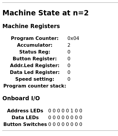
The final state of the “Hello World” program trace. The result of the computation (2) is in the Accumulator.

Note

This introduction to compilation via dgtools applies to any Digirule2 hardware. By default dgasm will produce a 2A executable but if you happen to have a different firmware installed (for example 2U) just specify it with parameter -g. For more information, please see the detailed script description.

Adding two literals saving the result to memory

Leaving the result of the addition in the accumulator is fine, but more commonly these results would have to be shifted out to some memory location (also known as a “variable”).

Our new listing is now:

# Implements the addition of two variables.
# This is equivalent to the statement `r3 = r0 + r1`.

COPYRA R0
ADDRA R1
COPYAR R3
HALT

R0:
.DB 1
R1:
.DB 1
R3:
.DB 0

Here, there are three labels (R0, R1, R2) that simply “tag” three locations in memory that hold initial literal values (1, 1 ,0 respectively).

These values are hard coded into the program here and will end up somewhere in memory. To get a full dump of the memory space at every time step of execution, we will need to run dgsim with an extra parameter.

The complete workflow is as follows:

> dgasm.py simpleadd_2.dsf
> dgsim.py simpleadd_2.dgb --with-dump

That second line will generate simpleadd_2_trace.html. If you open it with your browser and scroll all the way to the end you can see that where before there was a zero, now there is a 2.

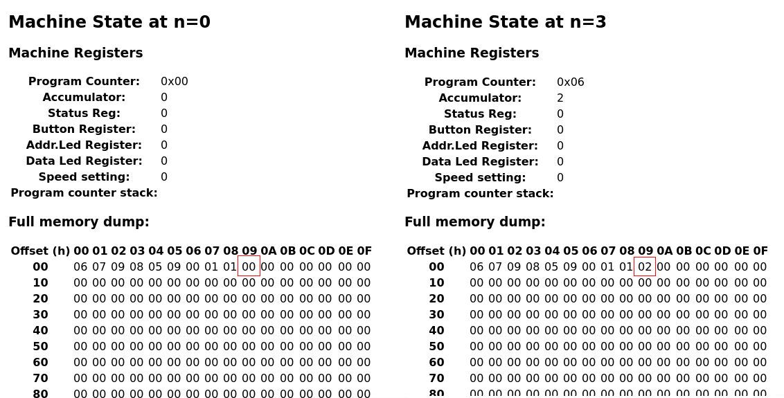
Initial and final states of the addition of two numbers. In this version, the result of the computation (2) has been shifted out to memory address 0x09 which started with an initial value of 0 and ended up with the value of 2. Also, notice the value of the Accumulator which is still 2, since it has not been cleared.

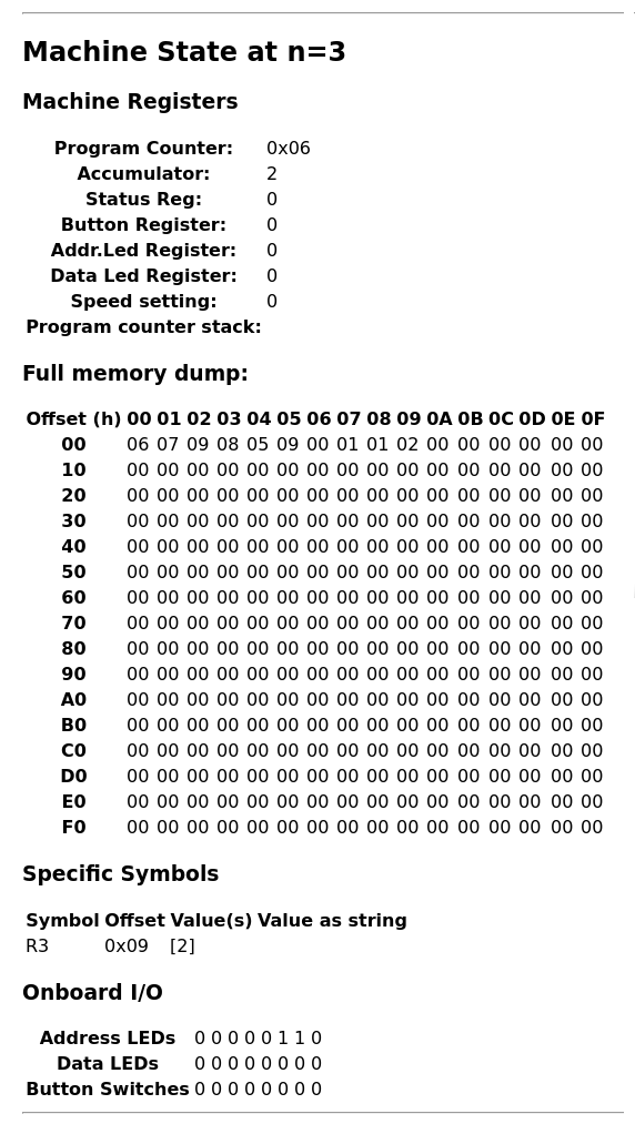
A more convenient way to monitor the values of specific memory locations (e.g. R3) is to tell dgsim to track that symbol throughout the execution of the program. This now helps in introducing the -ts parameter to dgsim:

> dgasm.py simpleadd_2.dsf
> dgsim.py simpleadd_2.dsf --with-dump -ts R3

Which produces a simpleadd_2_trace.html with all the changes of R3:

Introducing dginspect

This is a good point in the workflow to introduce the dginspect tool for inspecting already compiled programs and tracking labels.

dginspect provides a complete “dump” of a .dgb. archive. That is, it provides a complete listing of all the information about a given program that is captured within the .dgb archive.

It can be called by:

Which produces:

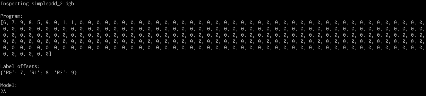
dginspect provides an X-Ray view of a .dgb archive, including a list of the defined labels and their offsets within Digirule’s memory.

For a more detailed explanation of how to use dginspect to track symbols, you might want to come back to this section in the appendix.

Adding two literals, sending the output to the Data LEDs

Certain registers of the Digirule 2 are memory mapped. For example, the Data LEDs are accessible at address 255. dgasm allows the definition of “symbols” that resolve to specific expressions. At the moment, “symbols” are used to define numeric constants, but in the future, these symbols might expand to whole expressions, akin to C’s macros.

Defining constants in this way does not take up any memory space. When the assembler comes across a “symbol”, it simply substitutes its value.

The code now is:

# Implements the addition of two constants.
# This is equivalent to the statement `r3 = a + b` 
# where `a` and `b` have been defined earlier
# as constants.
# Havin performed the addition, the result is also 
# sent to the display.
 
.EQU led_register=0xFF
.EQU a=1
.EQU b=1

COPYLA a
ADDLA b
COPYAR R3
COPYAR led_register
HALT
R3:
.DB 0

This program can be tried out in one of the ways that were explained previously.

Note

It would be useful to note here the difference between a “Label” and a “Symbol”. The value of a label is the address it points to in memory. The value of a symbol is the literal that was assigned to it through the .EQU directive.

Transfering the program to the Digirule

There are two ways to transfer your program to the Digirule, either via manually keying it in or transfering it via the serial port (on the Digirule 2U).

If you have a Digirule 2U, the transfer process is straightforward on Linux but involves a number of steps to identify and setup your serial communcations port. These are as follows:

If you don’t know which “device” your Digirule 2U uses:

1. Plug the Digirule 2U in

2. Find out which device file corresponds to the serial port

   1. The easiest way to do this is by > dmesg|egrep FTDI to which your OS will respond with something like [ 6093.755022] usb 2-2: FTDI USB Serial Device converter now attached to ttyUSB0.

   2. From this we know that the serial port the Digirule 2U is connected on is at /dev/ttyUSB0.

3. Make sure that you can write to the serial port

   1. By default, the serial port’s access rights might be restricted. But since we know that the only thing that is attached to this serial port is the Digirule 2U, we can go ahead and allow read/write access to it with: > sudo chmod o+rw /dev/ttyUSB0.

Once you know which “device” the Digirule 2U uses:

1. Set the communications port parameters

   1. The simplest way to do this is with > stty -F /dev/ttyUSB0 9600

2. Put the Digirule 2U in “programming mode” by holding down “Load” and “Next” on the device.

3. Send the .hex file

   • When you use dgasm.py with -g 2U, a .hex file containing the binary is also produced. To send it to the device, type > cat some_hex_file.hex>/dev/ttyUSB0 substituting of course for the .hex file you are trying to send and /dev/ttyUSB0 for the device the Digirule2U is identified as on your computer.

4. Click “Run” on the device.

To key the program in manually dginspect.py includes the -b option that “dumps” the complete assembled memory region as pairs of ADDR:VALUE values formatted in binary.

To key the program in, just make sure that a given memory address on the Digirule2 (indicated by the A0-7 LEDs) maps to the corresponding VALUE (indicated by the D0-7 LEDs).

To see what this looks like:

> dginspect.py simpleadd_3.dgb -b

This will simply dump everything to stdout, which means that it can be stored to be reviewed later with:

> dginspect.py simpleadd_3.dgb -b>add3_bin_output.txt

Or, if you are in Linux, simply send it to less with:

> dginspect.py simpleadd_3.dgb|less

In either case, the binary dump for simpleadd_3.dgb would look like this:

    ADDR:VALUE
00000000:00000100
00000001:00000001
00000010:00001000
00000011:00000001
00000100:00000101
00000101:00001001
00000110:00000101
00000111:11111111
00001000:00000000
00001001:00000000
00001010:00000000
00001011:00000000
...
...
...
...
...

Adding a literal and a user supplied input

The Digirule 2 has an elementary input device, a keyboard, attached to the CPU at address 253. Reading that “register” allows the program to read user input in the form of a binary number.

The Digirule 2 Virtual Machine includes a flexible mechanism that is called interactive mode that allows the simulation to take user input into account.

This is specified to dgsim with option -I.

The code listing for this example is as follows:

# Implements the addition of a constant plus a user defined 
# variable when this program is executed in interactive mode, 
# it is equivalent to `r3 = int(input()) + a`, where `a` has 
# already been defined as a constant ealier.

.EQU a=1
COPYLA a
ADDRA 253
COPYAR R3
HALT
R3:
.DB 0

The compilation process is now:

> dgasm.py simpleadd_4.dsf
> dgsim.py simpleadd_4.dgb -I

With -I, once the Digirule CPU tries to read from memory address 253 (or, 0xFD), a prompt will pop up for a binary input (i.e 0b00000010) which the program then adds 1 to and stores to the memory location labeled R3.

Here is the output with 0101 (i.e. 5), as the input.

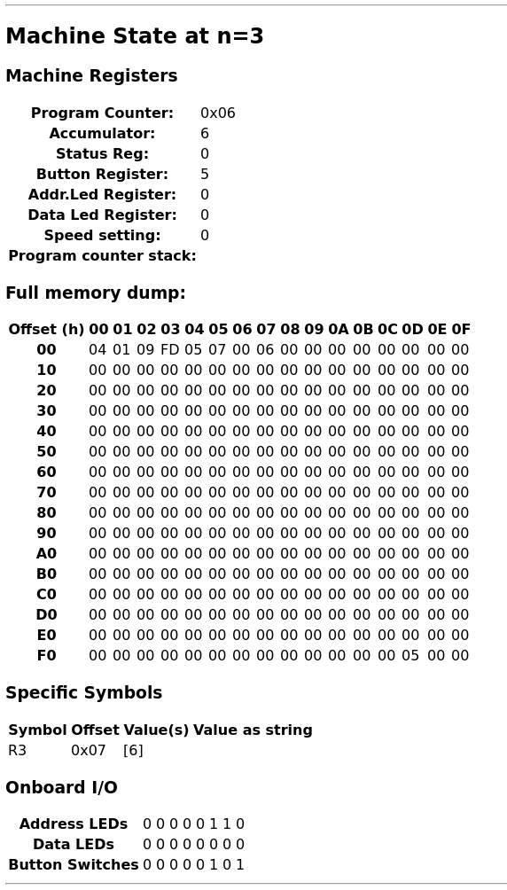
Passing 5 in interactive mode is visible at row 0xF0, column 0x0D (or address 0xFD). The program adds 1 and stores the value in R3.

Adding two literals with command line parametrisation

It probably has become apparent by now that dgsim can operate as a separate virtualised computing unit for Digirule hardware.

It can run programs and save its final state and it also provides ways of extracting those values from its memory space.

In fact, it is possible to parametrise Digirule 2 programs, call them and then extract values from the final memory space as follows:

# Implements `r3 = a + b`

COPYRA a
ADDRA b
COPYAR r3
HALT
R3:
.DB 0

a:
.DB 2
b:
.DB 6

This program specifies 1 byte a,b which hold literals that participate in addition and R3 that points to a one byte memory location that receives the result of the addition.

Very briefly, a,b will become the parameters (two numbers that can be reset without recompiling the program) and r3 will be the memory location that holds the final result.

The complete workflow is as follows, notice here which .dgb file is inspected for the results of the calculation:

1. Compile the program

   • > dgasm.py simpleadd_5.dsf

2. Run the program

   • > dgsim.py simpleadd_5.dgb

3. Inspect the result as stored in R3

   • > dginspect.py simpleadd_5_memdump.dgb -g r3

     • Notice here, we inspect the *_memdump.dgb file which is the final state of the program, at the end of the simulation.

   • With the program in its original form, this value should be 8.

4. Change parameter a to 3

   • > dginspect.py simpleadd_5.dgb -s 8 3

   • Don’t worry about overwriting simpleadd_5.dgb, its original form is still maintained in a .bak file.

   • Notice here that 8 is the offset of variable a

5. Run the program again

   • > dgsim.py simpleadd_5.dgb

6. Inspect the final result now

   • > dginspect.py simpleadd_5_memdump.dgb -g r3

   • With the parameters given here, this value should be 9

7. Start keying the final result in with:

   • > dginspect.py simpleadd_5_memdump.dgb -b

This is probably the most involved workflow using dgtools to take full control of program execution.

Each one of the three tools has more capabilities that were not expanded upon here but can be reviewed with --help. For more information please see section Detailed Script Descriptions.

With these points in mind, it is now time to move to advanced topics demonstrating more complex code on the Digirule 2.

---

Appendix:

Tracking symbols and dginspect

There is a little bit more to the way tracked symbols are specified. You can practically track the values of any region in memory, following the syntax -ts <symbol-name>[:Length[:Offset]]. Here is what this means:

1. -ts symbol-name

   • In this case, dgsim assumes that you are refering to an existing label defined in the program as a memory location that spans the length of just 1 Byte. If the label symbol-name does not exist in your program, this is flagged as an error.

2. -ts symbol-name:Length

   • Similar to the first case, but with this syntax, the length of memory that is tracked is Length bytes long (instead of the default 1). Again, the label symbol-name must be defined by your program, otherwise it is flagged as an error.

3. -ts symbol-name:Length:Offset

   • This is the most general case where any memory location that starts at Offset and spans Length bytes can be tracked. In this case, symbol-name is just a “tag” to differentiate tracked locations and it does not have to be defined by the program.

To discover the label names and their offsets as defined within a compiled program, you can use dginspect in the following way:

1. Compile the program:

   • > dgasm.py simpleadd_2.dsf

2. Use dginspect to obtain all defined symbols and their addresses:

   • > dginspect.py simpleadd_2.dgb

   • This produces:

     

     dginspect provides an X-Ray view of a .dgb archive, including a list of the defined labels and their offsets within Digirule’s memory.

3. Run dgsim telling it to “track” some symbols (e.g. R2, R3):

   • > dgsim.py simpleadd_2.dgb -ts R3 -ts R2

Adding multiple -ts options, keeps adding named references for dgsim to track. For example, suppose we wanted to track all three memory locations, then step 3 would become:

> dgsim.py simpleadd_2.dgb -ts R0 -ts R1 -ts R3

A complete example of the sort of output produced by dgsim for this file is availe through this link.